8. Tracking
- How does it work?
The matching step provides particle positions in 3D space for each frame. Then how to find particles trajectory? The simplest method is the closest neighbour method and is schematized in the figure below. Let’s take a particule \(P\) at time \(t\) (in black on the scheme). At time \(t+dt\) (red particles), we will look for the closest particle to \(P\) and will consider that it is the same particle (strond red particle). Doing that successively for all frames we will get the trajectory of particle \(P\).
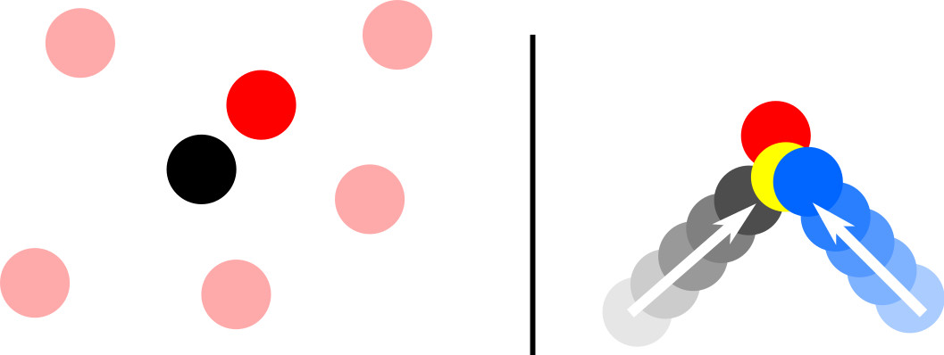
On the left, good tracking. On the right, typical tracking mistake.
However, when there are many particles in the flow, it is higly probable to do errors when other particles goes behing particle \(P\). This typical situation is represented on the right in the figure: particles two particles are tracked but when they become close this tracking method makes a mistake. The yellow particle is closer to the blue one so is attributed to the blue trajectory although it belongs to the black trajectory. To avoid that kind of mistakes, we do predictive tracking. For each time \(t\), we estimate the expected particle position thanks to previous particle position and then we look for the closest particle to the expected position.
General sketch of tracking. Two trajectories are shown here. Particles position for 5 successive frames are represented by crosses and their colour determines the time evolution.
The function track3d.m was made for that and requires 10 arguments:
session : Paths to the architecture root
ManipName : Name of the experiment
FileName : Name of the matched file without its extension (without .dat)
NbFrame : Number of frame in the file
maxdist : Maximum travelled distance between two successive frames
lmin : Minimum length of a trajectory (number of frames)
flag_pred : 1 for predictive tracking, 0 otherwise
npriormax : Maximum number of prior frames used for predictive tracking
flag_conf : 1 for conflict solving, 0 otherwise
minFrame : (optional) number of the first frame. Default = 1.

Input and output files of track3d.m function.
This function creates folders and calls track3d_manualfit.m function which estimates the next particle positions doing a manual fit instead of using polyfit function which is 30 times longer. The expected particle position is estimated using the last npriormax points. It creates a MATLAB structure and saves it as a file session.output_path/Processed_DATA/ManipName/tracks_%FileName.h5. This .h5 file can be openned with the function h52tracks.m` function which creates a MATLAB structure from the .h5 file. For each trajectory indexed by kt, the structure called here traj has the fields:
traj(kt).ntraj : trajectory index,
traj(kt).L : trajectory length,
traj(kt).frames : trajectory frames,
traj(kt).x : x-position,
traj(kt).y : y-position,
traj(kt).z : z-position,
traj(kt).nmatch : element indices in tracks.
Warning
It is also possible to do predictive tracking only when there are some conflict using track3d_polyfit.m function. For that, see the last lines of track3d.m function. track3d_polyfit.m function do closest neighbour tracking generally and predictive tracking only when two particles could belong to the same trajectory. In that case, called conflict situation, it uses polyfit function to estimate particle position. track3d_polyfit.m function provides very similar trajectories than track3d_manualfit.m with a difference of 0.1% in terms of number of trajectories. This difference reveals that less particules are lost with track3d_polyfit.m.
Note
To run tracking for test data:
session.input_path = "My4DPTVInstallationPath/Documentation/TestData/";  % My4DPTVInstallationPath has to be adapted !!!
session.output_path = "My4DPTVInstallationPath/Documentation/TestData/";
[tracks,traj]=track3d(session, "MyExperiment", "cam2_1-100",0.2,5,1,5,1);
To read output file:
traj = h52tracks("My4DPTVInstallationPath/Documentation/TestData/MyExperiment/tracks_matched_cam2_1-100");
Warning
How to run a compiled version of the track_3d.m?
It is possible to compile CenterFinding2D.m function to run it outside a MATLAB instance directly in a terminal. This can be useful to run it on cluster, for instance at the PSMN. The function to use for that is Arg_CenterFinding2D_PSMN.m.
- How to do?
Complete the header of the script
Arg_CenterFinding2D_PSMN.mto fill all required argument forCenterFinding2D.m. This script defines all arguments and callsCenterFinding2D.mfunction.Compile the script
Arg_CenterFinding2D_PSMN.mdoing in a matlab terminal:mcc -m Arg_CenterFinding2D_PSMN.m
An executable file
Arg_CenterFinding2D_PSMNwill appear in the same folder.To run it in your machine:
./Arg_CenterFinding2D_PSMN
To run it on the PSMN, you have to set the environment with the script
run_Arg_CenterFindingD_PSMN.sh. Write in a terminal:sh run_Arg_CenterFindingD_PSMN.sh $MCRROOT
Warning
To use PSMN installations see Tracking